Time series forecasting is a skill that few people claim to know. Machine learning is cool. And there are a lot of people interested in becoming a machine learning expert. But forecasting is something that is a little domain specific.
Retailers like Walmart, Target use forecasting systems and tools to replenish their products in the stores. An excellent forecast system helps in winning the other pipelines of the supply chain. If you are good at predicting the sale of items in the store, you can plan your inventory count well. You can plan your assortment well.
A good forecast leads to a series of wins in the other pipelines in the supply chain.
Disclaimer: The following post is my notes on forecasting which I have taken while having read several posts from Prof. Hyndman.
Let us get started. First things first.
What is time series?
A time series is a sequence of observations collected at some time intervals. Time plays an important role here. The observations collected are dependent on the time at which it is collected.
The sale of an item say Turkey wings in a retail store like Walmart will be a time series. The sale could be at daily level or weekly level. The number of people flying from Bangalore to Kolkata on daily basis is a time series. Time is important here. During Durga Puja holidays, this number would be humongous compared to the other days. This is know as seasonality.
What is the difference between a time series and a normal series?
Time component is important here. The time series is dependent on the time. However a normal series say 1, 2, 3...100 has no time component to it. When the value that a series will take depends on the time it was recorded, it is a time series.
How to define a time series object in R
ts() function is used for equally spaced time series data, it can be at any level. Daily, weekly, monthly, quarterly, yearly or even at minutes level. If you wish to use unequally spaced observations then you will have to use other packages.
ts() is used for numerical observations and you can set frequency of the data.
ts() takes a single frequency argument. There are times when there will be multiple frequencies in a time series. We use msts() multiple seasonality time series in such cases. I will talk about msts() in later part of the post. For now, let us define what is frequency.
Frequency
When setting the frequency, many people are confused what should be the correct value. This is the simple definition of frequency.
Frequency is the number of observations per cycle. Now, how you define what a cycle is for a time series?
Say, you have electricity consumption of Bangalore at hourly level. The cycle could be a day, a week or even annual. I will cover what frequency would be for all different type of time series.
Before we proceed I will reiterate this.
Frequency is the number of observations per cycle.
We will see what values frequency takes for different interval time series.
Daily data There could be a weekly cycle or annual cycle. So the frequency could be 7 or 365.25.
Some of the years have 366 days (leap years). So if your time series data has longer periods, it is better to use frequency = 365.25. This takes care of the leap year as well which may come in your data.
Weekly data
There could be an annual cycle.
frequency = 52 and if you want to take care of leap years then use frequency = 365.25/7
Monthly data
Cycle is of one year. So frequency = 12
Quarterly data Again cycle is of one year. So frequency = 4
Yearly data Frequency = 1
How about frequency for smaller interval time series
Hourly The cycles could be a day, a week, a year. Corresponding frequencies could be 24, 24 X 7, 24 X 7 X 365.25
Half-hourly The cycle could be a day, a week, a year. Corresponding frequencies could be 48, 48 X 7, 48 X 7 X 365.25
Minutes
The cycle could be hourly, daily, weekly, annual. Corresponding frequencies would be 60, 60 X 24, 60 X 24 X 7, 60 X 24 X 365.25
Seconds The cycle could be a minute, hourly, daily, weekly, annual. Corresponding frequencies would be 60, 60 X 60, 60 X 60 X 24,
60 X 60 X 24 X 7, 60 X 60 X 24 X 365.25
You might have observed, I have not included monthly cycles in any of the time series be it daily or weekly, minutes, etc. The short answer is, it is rare to have monthly seasonality in time series. To read more on this visit monthly-seasonality.
Now that we understand what is time series and how frequency is associated with it let us look at some practical examples.
Some useful packages
-
forecast: For forecasting functions
-
tseries: For unit root tests and GARC models
-
Mcomp: Time series data from forecasting competitions
-
fma: For data
-
expsmooth: For data
-
fpp: For data
We will now look at few examples of forecasting. We will look at three examples. Before that we will need to install and load this R package - fpp.
install.packages('fpp')
library(fpp)
Three examples
Sale of beer in Australia
dev.off() # to open up the plots with default settings.
ausbeer # is at quarterly level the sale of beer in each quarter.
plot(ausbeer)
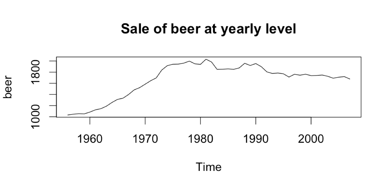
beer <- aggregate(ausbeer) # Converting to sale of beer at yearly level
plot(beer, main = 'Sale of beer at yearly level')
Sales of a group of pharmaceuticals
*a10 is a group of pharmaceuticals*
a10 # Sale of pharmaceuticals at monthly level from 1991 to 2008
head(a10)
plot(a10, main = 'Sale of pharmaceuticals at monthly level')
Electricity demand for a period of 12 weeks on daily basis
head(taylor)
plot(taylor)
Fully automated forecast
plot(forecast(beer))
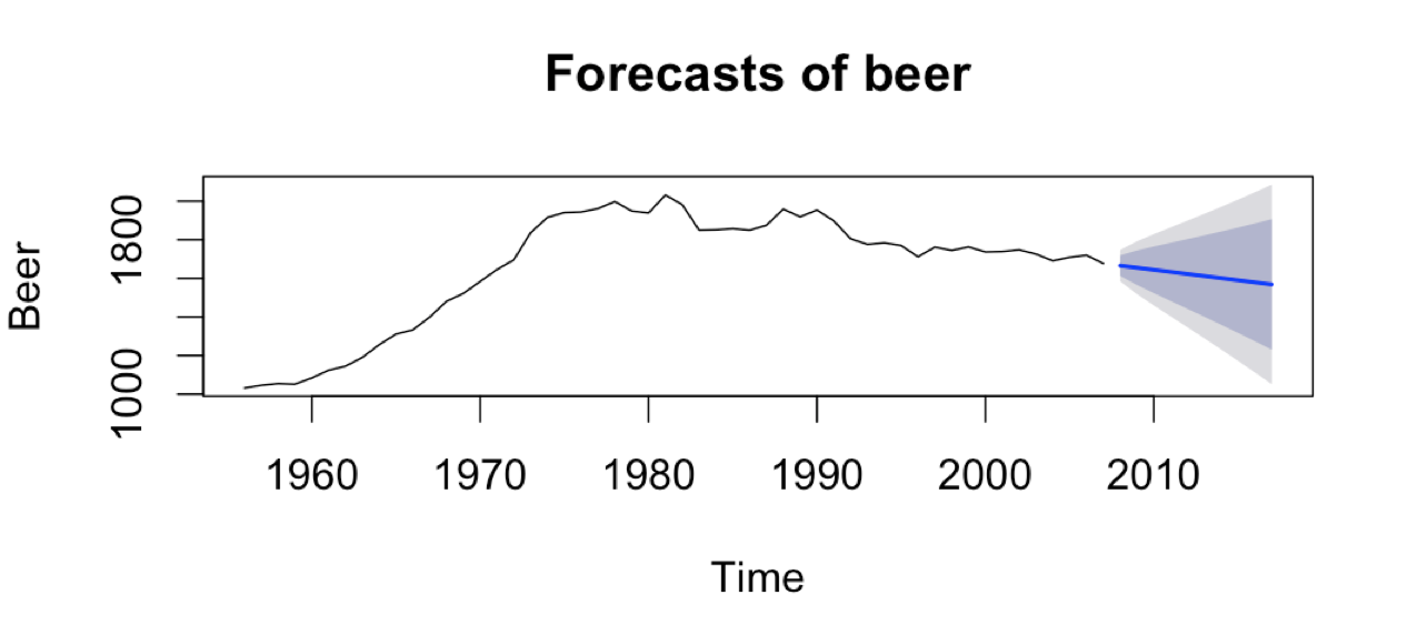
The blue line is a point forecast. You can see it has picked the annual trend. The inner shade is a 90% prediction interval and the outer shade is a 95% prediction interval.
Similar forecast plots for a10 and electricity demand can be plotted using
plot(forecast(a10))
plot(forecast(taylor))
Some simple forecasting methods
These are benchmark methods. You shouldn't use them. You will see why. These are naive and basic methods.
-
Mean method: Forecast of all future values is equal to mean of historical data Mean: meanf(x, h=10)
-
Naive method: Forecasts equal to last observed value Optimal for efficient stock markets naive(x, h=10) or rwf(x, h=10); rwf stands for random walk function
-
Seasonal Naive method: Forecast equal to last historical value in the same season snaive(x, h=10)
-
Drift method: Forecasts equal to last value plus average change Equivalent to extrapolating the line between the first and last observations rwf(x, drift = T, h=10)
Forecast objects in R
Functions that output a forecast object are:
-
meanf()
-
croston() Method used in supply chain forecast. For example to forecast the number of spare parts required in weekend
-
holt(), hw()
-
stlf()
-
ses() Simple exponential smoothing
Once you train a forecast model on a time series object, the model returns an output of forecast class that contains the following: -
Original series
-
Point forecasts
-
Prediction intervals
-
Forecasting method used
-
Residuals and in-sample one-step forecasts
A simple example on the beer time series
plot(beer)
fit <- ses(beer)
attributes(fit)
plot(fit)
Measures of forecast accuracy
-
MAE: Mean Absolute Error
-
MSE or RMSE: Mean Square Error or Root Mean Square Error
-
MAPE: Mean Absolute Percentage Error
MAE, MSE, RMSE are scale dependent.
MAPE is scale independent but is only sensible if the time series values >>0 for all i and y has a natural zero
Test methods on a test set
ausbeer # is at quarterly level the sale of beer in each quarter.
plot(ausbeer)
beer <- aggregate(ausbeer) # Converting to sale of beer at yearly level
plot(beer) # plot of yearly beer sales from 1956 to 2007

beer_train <- window(beer, end = 1994.99) # data from 1956 till 1994
plot(beer_train)

beer_test <- window(beer, start = 1995) # data from 1995 till 2007
plot(beer_test)

a10Train <- window(a10, end=2005.99)
a10Test <- window(a10, start = 2006)
Simple methods for the BEER data
f1 <- meanf(beer_train, h=8)
f2 <- rwf(beer_train, h=8)
f3 <- rwf(beer_train, drift = T, h = 8)

plot(f1)
plot(f2)
plot(f3)
In-sample accuracy
This will give you in-sample accuracy but that is not of much use. It just gives you an idea how will the model fit into the data. Chances are that the model may not fit well into the test data. So we should always look at the accuracy from the test data.
accuracy(f1)
accuracy(f2)
accuracy(f3)
Out-of-sample accuracy
accuracy(f1, beer_test)
accuracy(f2, beer_test)
accuracy(f3, beer_test)
Exponential smoothing
This method has been around since 1990s.
fit1 <- ets(beer_train, model = "ANN", damped = F)
fit2 <- ets(beer_train)

accuracy(fit1)
accuracy(fit2)

fcast1 <- forecast(fit1, h=8)
fcast2 <- forecast(fit2, h=8)
plot(fcast2)

accuracy(fcast1, beer_test)
accuracy(fcast2, beer_test)
General notation
ETS(Error, Trend, Seasonal) ETS(ExponenTial Smoothing)
ETS(X, Y, Z): 'X' stands for whether you add the errors or multiply the errors on point forecasts.
'Y' stands for whehter the trend component is additive or multiplicative or multiplicative damped
'Z' stands for whether the seasonal component is additive or multiplicative or multiplicative damped
Some examples
-
ETS(A, N, N): Simple exponential smoothing with additive errors 'A'/'M' stands for whether you add the errors on or multiply the errors on the point forecsats
-
ETS(A, A, N): HOlt's linear method with additive errors
-
ETS(A, A, A): Additive Holt-Winter's method with addtitive errors
-
ETS(M, A, M): Multiplicative Holt-Winter's method with multiplicative errors
There are 30 separate models in the ETS framework. However 11 of them are unstable so only 19 ETS models. So when you don't specify what model to use in model parameter, it fits all the 19 models and comes out with the best model using AIC criteria.
model1 <- ets(a10Train)
model2 <- ets(a10Train, model = 'MMM', damped = F)

forecast1 <- forecast(model1, h=30)
forecast2 <- forecast(model2, h=30)
There are many other parameters in the model which I suggest not to touch unless you know what you are doing. - Prof Hyndman
If you want to have a look at the parameters that the method chose. Just type in the name of your model.
model1
You will see the values of alpha, beta, gamma. Also,
sigma: the standard deviation of the residuals
AIC: Akaike Information criteria. AIC gives you and idea how well the model fits the data. ets fits all the 19 models, looks at the AIC and give the model with the lowest AIC. The lower the AIC, the better the model fits.
AICc: Corrected Akaike Information criteria
BIC: Bayesian Information Criteria
ets() function
-
Automatically chooses a model by default using the AIC, AICc, BIC
-
Can handle any combination of trend, seasonality and damping
-
Produces prediction intervals for every model
-
Ensures the parameters are admissible (equivalent to invertible)
-
Produces an object of class ets
ets objects -
Methods: coef(), plot(), summary(), residuals(), fitted(), simulate() and forecast()
-
plot() function shows the time plots of the original series along with the extracted components (level, growth and seasonal)
Automatic forecasting
Why use automatic forecasting?
-
Most users are not very expert at fitting time series models
-
Most experts cannot beat the best automatic algorithms. Prof. Hyndman accepted this fact for himself as well. He has been doing forecasting for the last 20 years.
-
Most busines need thousands of forecasts every week/month and they need it fast. You have to do it automatically.
-
Some multivariate forecasting methods depend on many univariate forecasts.
Box-Cox transformations
Transformations to stabilize the variance If the data show different variation at different levels of the series, then a transformation can be useful.
plot(a10)
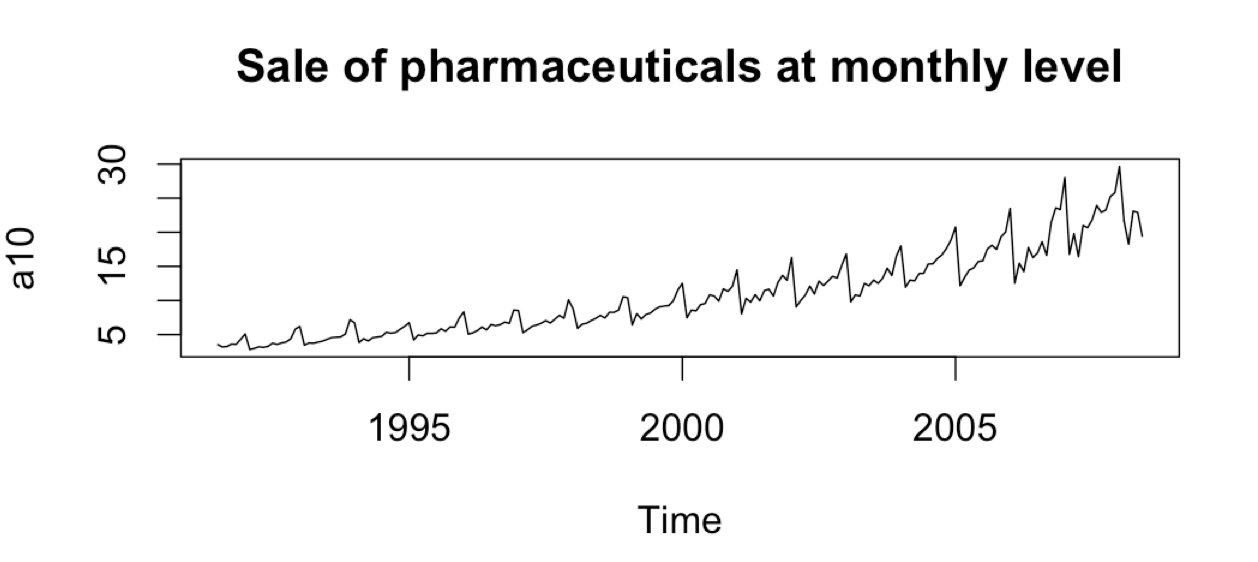
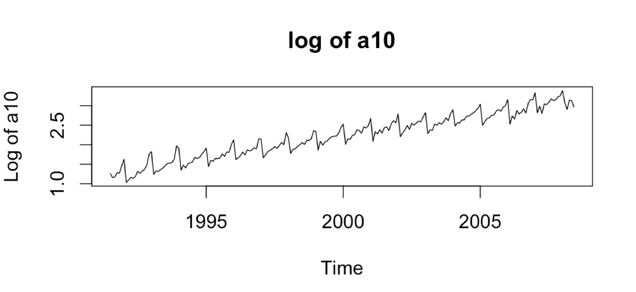
As you can see, the variation is increasing with the level of the series and the variation is multiplicative. If we take a log of the series, we will see that the variation becomes a little stable.
plot(log(a10), xlab = 'Time', ylab = 'Log of a10', main = 'log of a10')
Box-Cox transformations gives you value of parameter, lambda. And based on this value you decide if any transformation is needed or not.
-
lambda = 1 ; No substantive transformation
-
lambda = 1/2 ; Square root plus linear transformation
-
lambda = 0 ; Natural logarithm
-
lambda = -1; Inverse plus 1
Back-transformation
We must reverse the transformation (or back transform) to obtain forecasts on the original scale.
a10 # Sale of pharmaceuticals at monthly level from 1991 to 2008
plot(a10)
lam <- BoxCox.lambda(a10) # 0.131
lam
fit <- ets(a10, additive = T, lambda = lam)  # 'additive = T' implies we only want to consider additive models
plot(forecast(fit))
plot(forecast(fit), include=60)
ARIMA forecasting
R functions
-
The arima() function in the stats package provides seasonal and non-seasonal ARIMA model estimation including covariates
-
However, it does not allow a constant unless the model is stationary
-
It does not return everything required for forecast()
-
It does not allow re-fitting a model to new data
-
Use the Arima() function in the forecast package which acts as a wrapper to arima()
-
Or use auto.arima() function in the forecast package and it will find the model for you
This post was just a starter to time series. I will talk more about time series and forecasting in future posts. I plan to cover each of these methods - ses(), ets(), and Arima() in detail in future posts.
Did you find the article useful? If you did, share your thoughts in the comments. Share this post with people who you think would enjoy reading this. Let's talk more of data-science.